Kalman Filter

• parametric Bayesian filter
• algorithm for estimating the values of measured variables over time, given continuous measurements of those variables and the amount of uncertainty in those measurements
• estimate using past (possibly noisy) observations and present (and possibly noisy) observations

Assumptions

• noisy sensor
  • noise can be modelled using Gaussian Distribution PDF
• initial prior knowledge (state) is also a Gaussian Distribution PDF

Algorithm

1. Predict Step

predict the current state given the previous state and the time that has passed since

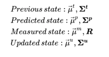
• state
  • prediction variable gaussian distribution
    • mean vector (of the prediction variable) and
    • covariance of prediction variables (uncertainity or noise in prediction variables)
  • e.g. mean and covariance of position and velocity of an object
• state-transition matrix (F): relates the previous state to the current one
• prediction equations
  • μ_p = F μ_t
    • μ_p = predicted mean vector
    • μ_t = mean vector at t
  • predicted covariance matrix
    • 
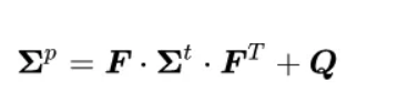
    • Q: process noise
      • encapsulates uncertainty created by the time that has passed since we last updated the state,

2. Update Step

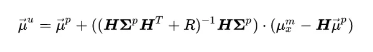
• combine the predicted state with an incoming measurement
• input two possible states and outputs a new state
•  Bayesian inference
• 
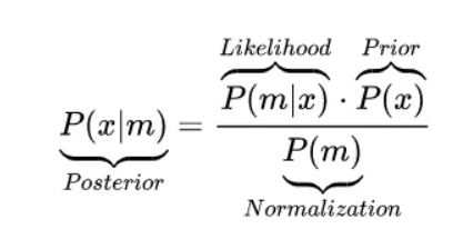
  • x = actual position
  • m = measured position
  • prior: predicted state
  • prior and likelihood are assumed to be Gaussian Distributions
  • Normalization i.e measurement probability distribution → empirically calculated
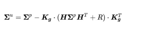
• Posterior probability (updated state) calculated is also a Gaussian Distribution
• 
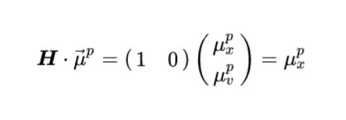
•  H → linear transformation that takes us from the state space to the measured space
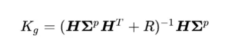
•  Kalman gain
  • factor by which we incorporate the new sensor information into the updated state
  • Error_estimate / (Error_estimate + Error_measured )
  • ( 0, 1)
    • 0 → estimate error =0 → estimate is perfect
    • 1 → measure error =0 → measure is perfect, estimate is imperfect

1-D case

Reference

• object tracking in 1-dimension
• assume constant velocity in 1-dimension
• let state = x, v → position, velocity
• 
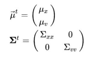
• initially there is no covariance between the velocity and position.
• Predict step equations
  • mean vector prediction
  • 
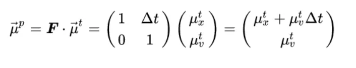
  • F picked based on constant velocity assumption
  • Solving for covariance
  • 
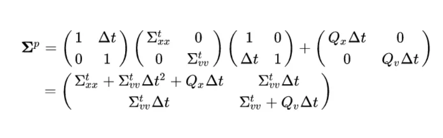
  • introduces off-diagonal elements in the covariance matrix
• Update Step equations
  • 
  • 
  • 
  • 

Pros

• updates are simple and efficient

Cons

• unimodal distribution
• class of motions restricted by linear model